if (!require("tidyverse")) install.packages("tidyverse")Data Wrangling Practice with R
R-Ladies Rome Tutorials
Introduction
Data preparation is a foundational step in the data science process. It refers to the set of procedures used to clean, organize, and structure data, ensuring it is ready for analysis. Without proper data preparation, even the most sophisticated analytical models can produce unreliable results due to inconsistencies or noise in the data. In practice, data preparation encompasses data wrangling, manipulation, and transformation techniques, which are essential for obtaining high-quality, actionable insights.
Essential Data Preparation Techniques: Wrangling, Manipulation, and Transformation
Data wrangling (also known as data munging) refers to the process of cleaning and organizing raw data to make it suitable for analysis. Data Wrangling also include data manipulation and transformation techniques that help to refine and structure the data for further analysis. These techniques are essential for ensuring data quality and consistency, enabling data scientists and analysts to derive meaningful insights from the data.
Data wrangling involves cleaning raw data handling missing values, correcting errors, and merging datasets—to ensure accuracy and consistency. It also includes structuring data into a tidy format, where each variable is a column, each observation is a row, and each type of observational unit is a table. This format makes it easier to analyze and visualize data effectively.
- Handling Missing Data: Missing values (NA) are common in datasets. R provides several ways to address them, such as using is.na() to detect them, and na.omit() to remove them, or applying imputation methods to fill in missing values.
- Dealing with Duplicates: Identifying and removing duplicate rows is essential to avoid skewed results. The distinct() function in R’s dplyr package makes this task simple.
- Standardizing Data Formats: Ensuring consistent data types is crucial, especially for numeric, character, and factor variables. Functions like mutate() and as.numeric(), as.character(), or as.factor() help transform data into the appropriate format.
Data manipulation builds on this by adjusting, filtering, and transforming specific aspects of the data, such as selecting relevant columns, filtering rows based on conditions, and creating new variables.
- Filtering Data: Filtering allows you to extract specific rows based on conditions. The filter() function in dplyr is useful for this task.
- Sorting Data: Sorting data helps organize it in a meaningful way. The arrange() function in dplyr can sort data by one or more columns.
- Grouping Data: Grouping data allows you to perform calculations on subsets of the data. The group_by() function in dplyr is used to group data by one or more variables.
- Summarizing Data: Summarizing data provides insights into the dataset’s characteristics. The summarize() function in dplyr can calculate summary statistics like mean, median, and standard deviation.
Data transformation goes deeper by reshaping the structure of the data (e.g., converting between wide and long formats), normalizing values, or applying mathematical operations like log transformations to ensure that the data is suitable for complex analysis or modeling.
- Reshaping Data: Reshaping data involves converting between wide and long formats using functions like gather() and spread() in tidyr.
- Normalizing Data: Normalizing data involves scaling values to a standard range, such as between 0 and 1, to ensure consistency across variables.
- Applying Mathematical Operations: Mathematical operations like log transformations, standardization, or normalization can help prepare data for advanced analyses like machine learning.
These processes, often performed using R packages like dplyr, tidyr, and data.table, are crucial steps in converting raw, disorganized data into meaningful insights. Together, they form the foundation for effective data analytics, which uses cleaned and well-structured data to perform descriptive, predictive, and inferential analyses.
Practice with Cardio Data
The data we will be working with is the cardio_train.csv dataset, which contains information on patients with cardiovascular disease. It can be found on Kaggle at the following link: Cardiovascular Disease Dataset.
Data Description
The dataset includes the following columns:
| Column Name | Description | Variable Name | Data Type |
|---|---|---|---|
| Age | Objective Feature | age | int (days) |
| Height | Objective Feature | height | int (cm) |
| Weight | Objective Feature | weight | float (kg) |
| Gender | Objective Feature | gender | categorical (1 w, 2 m) |
| Systolic blood pressure | Examination Feature | ap_hi | int |
| Diastolic blood pressure | Examination Feature | ap_lo | int |
| Cholesterol | Examination Feature | cholesterol | 1: normal, 2: above normal, 3: well above normal |
| Glucose | Examination Feature | gluc | 1: normal, 2: above normal, 3: well above normal |
| Smoking | Subjective Feature | smoke | binary |
| Alcohol intake | Subjective Feature | alco | binary |
| Physical activity | Subjective Feature | active | binary |
| Presence or absence of cardiovascular disease | Target Variable | cardio | binary |
Libraries and Data
Install the package if is not already installed:
Load the tidyverse package:
library(tidyverse)Import Data
Unzip the file in the data folder:
unzip("data/cardio_train.zip", exdir = "data")We load the dataset using the read.csv function part of the base R package and used to read comma-separated values (CSV) files. It allows us to use the sep = ";" option, which is necessary for reading the cardio_train.csv file.
?utils::read.csvcardio_train <- read.csv("data/cardio_train.csv", sep=";")Inspect Data
head(cardio_train) id age gender height weight ap_hi ap_lo cholesterol gluc smoke alco active
1 0 18393 2 168 62 110 80 1 1 0 0 1
2 1 20228 1 156 85 140 90 3 1 0 0 1
3 2 18857 1 165 64 130 70 3 1 0 0 0
4 3 17623 2 169 82 150 100 1 1 0 0 1
5 4 17474 1 156 56 100 60 1 1 0 0 0
6 8 21914 1 151 67 120 80 2 2 0 0 0
cardio
1 0
2 1
3 1
4 1
5 0
6 0cardio_train %>% glimpse()Rows: 70,000
Columns: 13
$ id <int> 0, 1, 2, 3, 4, 8, 9, 12, 13, 14, 15, 16, 18, 21, 23, 24, 2…
$ age <int> 18393, 20228, 18857, 17623, 17474, 21914, 22113, 22584, 17…
$ gender <int> 2, 1, 1, 2, 1, 1, 1, 2, 1, 1, 1, 2, 2, 1, 2, 2, 1, 1, 1, 2…
$ height <int> 168, 156, 165, 169, 156, 151, 157, 178, 158, 164, 169, 173…
$ weight <dbl> 62, 85, 64, 82, 56, 67, 93, 95, 71, 68, 80, 60, 60, 78, 95…
$ ap_hi <int> 110, 140, 130, 150, 100, 120, 130, 130, 110, 110, 120, 120…
$ ap_lo <int> 80, 90, 70, 100, 60, 80, 80, 90, 70, 60, 80, 80, 80, 70, 9…
$ cholesterol <int> 1, 3, 3, 1, 1, 2, 3, 3, 1, 1, 1, 1, 1, 1, 1, 1, 1, 1, 1, 1…
$ gluc <int> 1, 1, 1, 1, 1, 2, 1, 3, 1, 1, 1, 1, 1, 1, 1, 1, 1, 3, 1, 1…
$ smoke <int> 0, 0, 0, 0, 0, 0, 0, 0, 0, 0, 0, 0, 0, 0, 1, 0, 0, 0, 0, 1…
$ alco <int> 0, 0, 0, 0, 0, 0, 0, 0, 0, 0, 0, 0, 0, 0, 1, 0, 0, 0, 0, 0…
$ active <int> 1, 1, 0, 1, 0, 0, 1, 1, 1, 0, 1, 1, 0, 1, 1, 0, 0, 1, 0, 1…
$ cardio <int> 0, 1, 1, 1, 0, 0, 0, 1, 0, 0, 0, 0, 0, 0, 0, 1, 0, 0, 0, 0…This dataset contains 70000 observations and 13 variables. The variables include age (in days), height (in cm), weight (in kg), and others that describe the patients’ health status and lifestyle factors.
Data Wrangling
Handling Missing Data
is.na()na.omit()drop_na()
cardio_train %>% is.na() %>% colSums() id age gender height weight ap_hi
0 0 0 0 0 0
ap_lo cholesterol gluc smoke alco active
0 0 0 0 0 0
cardio
0 There are no missing values in this dataset.
Dealing with Duplicates
distinct()
cardio_train %>% dim()[1] 70000 13cardio_train %>% distinct() %>% nrow()[1] 70000Rename original data cardio_train to cardio for easier reference, and as a best practice to keep the original data intact:
cardio <- cardio_trainStandardizing Data Formats
mutate()as.numeric()as.character()as.factor()
Depending on the type of analysis we want to perform, we may need to convert the age variable from days to years. Let’s see how we can create a new variable age_years that represents the age in years, we can use the round function to round the age in years to the nearest whole number:
cardio %>%
  mutate(age_years = round(age / 365.25),
         .after = age) %>%
  head()
id age age_years gender height weight ap_hi ap_lo cholesterol gluc smoke
1 0 18393 50 2 168 62 110 80 1 1 0
2 1 20228 55 1 156 85 140 90 3 1 0
3 2 18857 52 1 165 64 130 70 3 1 0
4 3 17623 48 2 169 82 150 100 1 1 0
5 4 17474 48 1 156 56 100 60 1 1 0
6 8 21914 60 1 151 67 120 80 2 2 0
alco active cardio
1 0 1 0
2 0 1 1
3 0 0 1
4 0 1 1
5 0 0 0
6 0 0 0Data Manipulation
Subsetting Data
select()filter()
Let’s select a subset of columns from the dataset:
cardio %>%
  mutate(age_years = round(age / 365.25)) %>%
  select(age, age_years) %>%
  head()
age age_years
1 18393 50
2 20228 55
3 18857 52
4 17623 48
5 17474 48
6 21914 60Let’s filter a subset of columns from the dataset:
cardio %>%
  mutate(age_years = round(age / 365.25)) %>%
  select(age, age_years) %>%
  filter(age_years > 50) %>%
  head()
age age_years
1 20228 55
2 18857 52
3 21914 60
4 22113 61
5 22584 62
6 19834 54Grouping and Summarizing Data
group_by()summarize()
cardio %>%
  mutate(age_years = round(age / 365.25)) %>%
  group_by(cholesterol) %>%
  summarize(mean_age = round(mean(age_years, na.rm = TRUE)),
            mean_weight = mean(weight, na.rm = TRUE),
            median_height = median(height, na.rm = TRUE)) %>%
  head()
# A tibble: 3 × 4
cholesterol mean_age mean_weight median_height
<int> <dbl> <dbl> <dbl>
1 1 53 73.1 165
2 2 54 76.7 164
3 3 56 78.8 163Creating New Variables
mutate()
Let’s create a new variable bmi (Body Mass Index) by calculating the weight in kilograms divided by the square of the height in meters:
cardio %>%
  mutate(age_years = round(age / 365.25),
         bmi = weight / ((height / 100) ^ 2)) %>%
  select(cardio, age_years, weight, height, bmi, cholesterol) %>%
  head()
cardio age_years weight height bmi cholesterol
1 0 50 62 168 21.96712 1
2 1 55 85 156 34.92768 3
3 1 52 64 165 23.50781 3
4 1 48 82 169 28.71048 1
5 0 48 56 156 23.01118 1
6 0 60 67 151 29.38468 2Let’s filter the dataset to include only patients with a BMI greater than 30 (obese patients):
cardio %>%
  mutate(age_years = round(age / 365.25),
         bmi = weight / ((height / 100) ^ 2)) %>%
  select(cardio, age_years, weight, height, bmi, cholesterol)  %>%
  filter(bmi > 30) %>%
  head()
cardio age_years weight height bmi cholesterol
1 1 55 85 156 34.92768 3
2 0 61 93 157 37.72973 3
3 0 54 78 158 31.24499 1
4 1 46 112 172 37.85830 1
5 0 54 83 163 31.23941 1
6 1 63 90 158 36.05191 2cardio %>%
mutate(gender = factor(gender,
levels = c('female' = 1, 'male' = 2),
labels = c('female', 'male')),
bmi = weight / ((height / 100) ^ 2)) %>%
ggplot(aes(x = bmi, fill = gender)) +
geom_histogram(binwidth = 2) +
xlim(0, 100) +
labs(title = "BMI Distribution by Gender",
x = "BMI",
y = "Count") 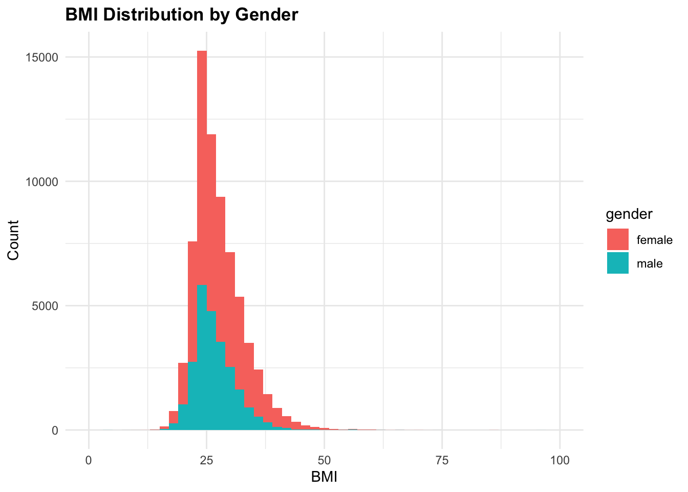
Sorting Data
arrange()
Let’s sort the dataset by age in descending order:
cardio %>%
  mutate(age_years = round(age / 365.25)) %>%
  arrange(desc(age)) %>%
  select(age, age_years) %>%
  head()
age age_years
1 23713 65
2 23701 65
3 23692 65
4 23690 65
5 23687 65
6 23684 65More Grouping
group_by()summarize()
Let’s group the data by cardio, and age in years and calculate the average BMI for each age group:
cardio %>%
  mutate(age_years = round(age / 365.25),
         bmi = weight / ((height / 100) ^ 2)) %>%
  group_by(cardio, age_years) %>%
  summarize(avg_bmi = mean(bmi, na.rm = TRUE)) %>%
  head()
# A tibble: 6 × 3
# Groups: cardio [1]
cardio age_years avg_bmi
<int> <dbl> <dbl>
1 0 30 23.9
2 0 39 26.3
3 0 40 25.7
4 0 41 25.9
5 0 42 25.7
6 0 43 26.0cardio %>%
mutate(age_years = round(age / 365.25),
bmi = weight / ((height / 100) ^ 2),
cardio = factor(cardio, labels = c("CVD", "NO CVD"))) %>%
group_by(cardio, age_years) %>%
summarize(avg_bmi = mean(bmi, na.rm = TRUE)) %>%
ggplot(aes(x = age_years, y = avg_bmi)) +
geom_point() +
geom_smooth(linewidth = 0.5,
linetype = "dashed",
se = F) +
facet_wrap( ~ cardio, scales = "free")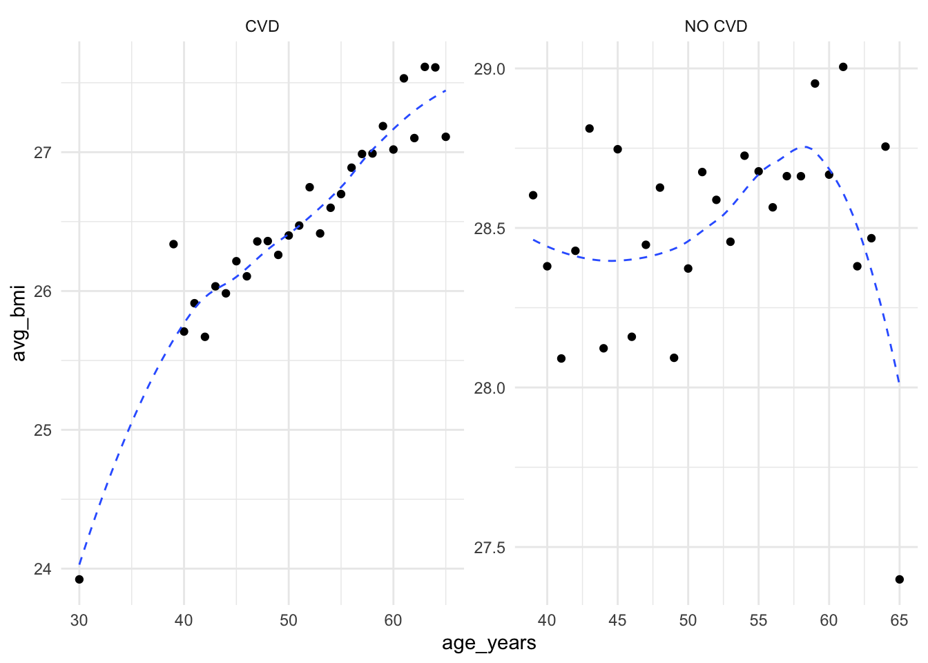
Summary Statistics
summary()
Let’s calculate the summary statistics for the all variables:
cardio %>%
  mutate(age_years = round(age / 365.25),
         bmi = weight / ((height / 100) ^ 2),
         .after = age) %>%
  map_df(~summary(.), .id = "var") %>%
  column_to_rownames(var = "var") %>%
  janitor::clean_names() %>%
  mutate(mean = round(mean)) %>%
  relocate(mean, median, min, max)
mean median min max x1st_qu x3rd_qu
id 49972 50001.50000 0.000000 99999.0000 25006.75000 74889.25000
age 19469 19703.00000 10798.000000 23713.0000 17664.00000 21327.00000
age_years 53 54.00000 30.000000 65.0000 48.00000 58.00000
bmi 28 26.37407 3.471784 298.6667 23.87511 30.22222
gender 1 1.00000 1.000000 2.0000 1.00000 2.00000
height 164 165.00000 55.000000 250.0000 159.00000 170.00000
weight 74 72.00000 10.000000 200.0000 65.00000 82.00000
ap_hi 129 120.00000 -150.000000 16020.0000 120.00000 140.00000
ap_lo 97 80.00000 -70.000000 11000.0000 80.00000 90.00000
cholesterol 1 1.00000 1.000000 3.0000 1.00000 2.00000
gluc 1 1.00000 1.000000 3.0000 1.00000 1.00000
smoke 0 0.00000 0.000000 1.0000 0.00000 0.00000
alco 0 0.00000 0.000000 1.0000 0.00000 0.00000
active 1 1.00000 0.000000 1.0000 1.00000 1.00000
cardio 0 0.00000 0.000000 1.0000 0.00000 1.00000Let’s calculate the summary statistics for the numeric variables only:
cardio %>%
  mutate(id = row.names("id"),
         gender = as.factor(gender),
         smoke = as.factor(smoke),
         active = as.factor(active),
         cardio = as.factor(cardio)) %>%
  # summarize stats only for numeric variables
  summarize(across(where(is.numeric),
                   list(mean = mean,
                        median = median,
                        sd = sd))) %>%
  t()
[,1]
age_mean 1.946887e+04
age_median 1.970300e+04
age_sd 2.467252e+03
height_mean 1.643592e+02
height_median 1.650000e+02
height_sd 8.210126e+00
weight_mean 7.420569e+01
weight_median 7.200000e+01
weight_sd 1.439576e+01
ap_hi_mean 1.288173e+02
ap_hi_median 1.200000e+02
ap_hi_sd 1.540114e+02
ap_lo_mean 9.663041e+01
ap_lo_median 8.000000e+01
ap_lo_sd 1.884725e+02
cholesterol_mean 1.366871e+00
cholesterol_median 1.000000e+00
cholesterol_sd 6.802503e-01
gluc_mean 1.226457e+00
gluc_median 1.000000e+00
gluc_sd 5.722703e-01
alco_mean 5.377143e-02
alco_median 0.000000e+00
alco_sd 2.255677e-01Data Transformation
Combining Datasets
left_join()inner_join()right_join()full_join()bind_rows()/bind_cols()merge()
In some cases, we may need to combine multiple datasets to perform more complex analyses. We can use one of the join functions from the dplyr package to join two datasets based on a common key.
cardio %>%
  mutate(age_years = round(age / 365.25)) %>%
  pull(age_years) %>%
  summary()
Min. 1st Qu. Median Mean 3rd Qu. Max.
30.0 48.0 54.0 53.3 58.0 65.0 Let’s group age by intervals and count the number of observations in each group:
cardio %>%
  mutate(id = row.names("id"),
         age_years = round(age / 365.25),
         # group age_years in intervals and assign it to a new variable
         age_group = cut_interval(age_years,
                                  n = 4,
                                  labels = c("5-14", "15-49", "50-69", "70+")),
         .after = age) %>%
  arrange(age_years) %>%
  count(age_group)
age_group n
1 5-14 4
2 15-49 14569
3 50-69 31137
4 70+ 24290Let’s create a new dataset cardio2 by adding a new variable bmi, other transformations to the original dataset cardio:
cardio2 <- cardio %>%
  mutate(id = row.names("id"),
         age_years = round(age / 365.25),
         age_group = cut_interval(age_years,
                                  n = 4,
                                  labels = c("5-14", "15-49",
                                             "50-69","70+")),
         bmi = weight / ((height / 100) ^ 2),
         cardio = factor(cardio, levels = c(0,1)),
         gender = factor(gender,
                         levels = c(1,2),
                         labels = c("female", "male")),
         smoke = factor(smoke, levels = c(0,1))) %>%
  select(cardio, age_group, gender,
         weight, height, smoke,
         cholesterol, gluc, bmi)  %>%
  filter(bmi > 30) %>%
  distinct()
And now create cardio3 dataset with the mean values for bmi, weight, height, and the count of observations for each group:
cardio3 <- cardio2 %>%
  group_by(cardio, age_group, gender, smoke, cholesterol, gluc) %>%
  reframe(mean_bmi = mean(bmi, na.rm = TRUE),
          mean_weight = mean(weight, na.rm = TRUE),
          mean_height = mean(height, na.rm = TRUE),
          count = n())
cardio3 %>% head()# A tibble: 6 × 10
cardio age_group gender smoke cholesterol gluc mean_bmi mean_weight
<fct> <fct> <fct> <fct> <int> <int> <dbl> <dbl>
1 0 5-14 male 0 1 1 30.0 92
2 0 15-49 female 0 1 1 36.0 90.3
3 0 15-49 female 0 1 2 34.6 87.4
4 0 15-49 female 0 1 3 35.6 90.6
5 0 15-49 female 0 2 1 35.3 89.2
6 0 15-49 female 0 2 2 34.6 90.6
# ℹ 2 more variables: mean_height <dbl>, count <int>Let’s join the cardio3 with a new dataset cardio_deaths with the deaths rates due to cardiovascular diseases by country and year, data is from the IHME website:
cardio_deaths <- read_csv("data/cardio_deaths.csv")
cardio_deaths %>% head()
# A tibble: 6 × 5
location year age gender value
<chr> <dbl> <chr> <chr> <dbl>
1 Low SDI 1990 15-49 female 34.7
2 Low SDI 1991 15-49 female 34.4
3 Low SDI 1992 15-49 female 34.1
4 Low SDI 1993 15-49 female 33.8
5 Low SDI 1994 15-49 female 33.7
6 Low SDI 1995 15-49 female 33.4Let’s check the dimensions of the cardio3 and cardio_deaths datasets:
cardio3 %>% dim();[1] 200 10cardio_deaths %>% dim()[1] 1280 5Let’s join the cardio3 and cardio_deaths datasets using the right_join function from the dplyr package:
cardio_join <- cardio_deaths %>%
  group_by(age, gender) %>%
  reframe(avg_deaths = mean(value, na.rm = TRUE)) %>%
  right_join(cardio3,
            by = c("age" = "age_group", "gender"))
Let’s check the dimensions of the joined dataset and the number of distinct rows:
cardio_join %>% dim;[1] 200 11cardio_join %>% distinct() %>% dim()[1] 200 11Let’s check the first few rows of the joined dataset:
head(cardio_join)# A tibble: 6 × 11
age gender avg_deaths cardio smoke cholesterol gluc mean_bmi mean_weight
<chr> <chr> <dbl> <fct> <fct> <int> <int> <dbl> <dbl>
1 15-49 female 24.8 0 0 1 1 36.0 90.3
2 15-49 female 24.8 0 0 1 2 34.6 87.4
3 15-49 female 24.8 0 0 1 3 35.6 90.6
4 15-49 female 24.8 0 0 2 1 35.3 89.2
5 15-49 female 24.8 0 0 2 2 34.6 90.6
6 15-49 female 24.8 0 0 2 3 31.2 72
# ℹ 2 more variables: mean_height <dbl>, count <int>Tidying Data
pivot_longer()pivot_wider()gather()- the same aspivot_longer()spread()- the same aspivot_wider()separate()unite()
Let’s pivot the cardio_join dataset from wide to long format to separate the cholesterol and gluc variables into a single column exam_type and a single column result:
cardio_join_long <- cardio_join %>%
  pivot_longer(cols = c(cholesterol, gluc),
               names_to = "exam_type",
               values_to = "result") %>%
  select(cardio, age, exam_type, result)

cardio_join_long %>%
  head()
# A tibble: 6 × 4
cardio age exam_type result
<fct> <chr> <chr> <int>
1 0 15-49 cholesterol 1
2 0 15-49 gluc 1
3 0 15-49 cholesterol 1
4 0 15-49 gluc 2
5 0 15-49 cholesterol 1
6 0 15-49 gluc 3Let’s check the dimensions of the cardio_join_long dataset and the number of distinct rows:
cardio_join_long %>% dim();[1] 400 4cardio_join_long %>% distinct() %>% dim()[1] 38 4Let’s remove duplicate rows from the cardio_join_long dataset:
cardio_join_long <- cardio_join_long %>%
  distinct()
Let’s pivot the cardio_join_long dataset back to the original format:
cardio_join_long %>%
  group_by(cardio, age) %>%
  pivot_wider(names_from = exam_type,
              values_from = result) %>%
  # unlist the nested columns
  unnest(cols = c(cholesterol, gluc)) %>%
  head()
# A tibble: 6 × 4
# Groups: cardio, age [2]
cardio age cholesterol gluc
<fct> <chr> <int> <int>
1 0 15-49 1 1
2 0 15-49 2 2
3 0 15-49 3 3
4 1 15-49 1 1
5 1 15-49 2 2
6 1 15-49 3 3And, let’s separate the age variable into two columns age_group_start and age_group_end:
cardio_join_age_group_sep <- cardio_join %>%
  separate(col = "age",
           into = c("age_group_start", "age_group_end"),
           remove = F) %>%
  select(cardio, age_group_start, age_group_end)

cardio_join_age_group_sep %>%
  head()
# A tibble: 6 × 3
cardio age_group_start age_group_end
<fct> <chr> <chr>
1 0 15 49
2 0 15 49
3 0 15 49
4 0 15 49
5 0 15 49
6 0 15 49 Then, let’s unite the age_group_start and age_group_end columns back into a single column age:
cardio_join_age_group_sep %>%
  unite(col = "age",
        age_group_start, age_group_end, sep = "-") %>%
  select(cardio, age) %>%
  head()
# A tibble: 6 × 2
cardio age
<fct> <chr>
1 0 15-49
2 0 15-49
3 0 15-49
4 0 15-49
5 0 15-49
6 0 15-49Exporting Data
write.csv()
Once we have cleaned and transformed the data, we may want to export it to a file for further analysis or sharing. We can use the write.csv function to export the data to a CSV file.
Let’s export the cardio_join dataset to a CSV file named cardio_cleaned.csv:
write.csv(cardio_join, "data/cardio_cleaned.csv", row.names = FALSE)Summary
Data wrangling, manipulation, and transformation are essential techniques for preparing and refining data for analysis. By cleaning, transforming, and organizing raw data, we can ensure its accuracy and consistency, making it suitable for analysis and visualization. These processes form the foundation for effective data analytics, enabling us to derive meaningful insights and make informed decisions based on the data.
In this tutorial, we explored various data wrangling techniques using the cardio_train.csv dataset, including checking for missing values, transforming variables, filtering and sorting data, grouping data, and calculating summary statistics. By applying these techniques, we gained valuable insights into the dataset and learned how to manipulate and analyze data effectively using R.
Data wrangling is a critical skill for data scientists and analysts, as it allows them to work with raw data and prepare it for analysis. By mastering these techniques, you can ensure that your data is clean, well-structured, and ready for further analysis, enabling you to derive meaningful insights and make informed decisions based on the data.
References
- Cardiovascular Disease Dataset on Kaggle
- IHME website
- R for Data Science by Wickham, H., & Grolemund, G. (2017). O’Reilly Media.
- Tidyverse Learn Documentation
- Tidy Data by Wickham, H. (2014). Journal of Statistical Software, 59(10), 1-23